Whiteboard Technical Series: Decision Trees
Decision trees: Why they’re so effective at troubleshooting network issues.
In this third installment of the Juniper Whiteboard Technical Series, you'll see how the Juniper/Mist AI platform uses Decision Tree models to identify common networking problems.
You’ll learn
How Decision Trees pinpoint common network issues, like faulty cables, access point and switch problems, plus wireless coverage
How to isolate a cable fault by creating a Decision Tree using features of a bad cable, such a frame errors and one-way traffic
How the structure of a Decision Tree accomplishes the ultimate goal: to produce an accurate model with a high level of certainty
Who is this for?
Transcript
0:11 today we'll be looking at decision trees
0:13 and how they identify common network
0:15 issues like faulty network cables
0:17 ap or switch health and wireless
0:19 coverage
0:20 the algorithms used include simple
0:23 random forest
0:24 gradient boosting and xg boost
0:27 our example will be a simple decision
0:29 tree algorithm
0:31 the essential steps in any machine
0:33 learning project involve collecting data
0:36 training a model then deploying that
0:38 model
0:39 decision trees are no different let's
0:41 use a real world example
0:44 in networking decision trees can be
0:46 applied to incomplete negotiation
0:48 detection
0:49 mtu mismatch among others our example
0:52 today applies the fundamental problem of
0:54 determining cable faults
0:56 a cable is neither 100 good nor bad
0:59 but somewhere in between to isolate a
1:02 fault we can create a decision tree
1:04 using features of a bad cable such as
1:06 frame errors and one-way traffic
1:09 we begin a decision tree by asking a
1:12 question which will have the greatest
1:13 impact on label separation
1:16 we use two metrics to determine that
1:18 question genie impurity
1:20 and information gain genie impurity
1:23 which is similar to entropy
1:25 determines how much uncertainty there is
1:27 in a node and information gain lets us
1:29 calculate
1:30 how much a question reduces that
1:32 uncertainty
1:33 a decision tree is based on a data set
1:35 from known results
1:37 each row is an example the first two
1:40 columns are features that describe the
1:42 label in the final column
1:43 a good or bad cable the data set can be
1:46 modified to add additional features
1:48 and the structure will remain the same a
1:52 decision tree starts with a single root
1:53 node which is given this full training
1:55 set
1:57 the node will then ask a yes no question
1:59 about one of the features
2:00 and split into two subsets of data which
2:02 is now the input of a child node
2:05 if the labels are still mixed good and
2:07 bad
2:08 then another yes no question will be
2:10 asked
2:12 the goal of a decision tree is to sort
2:13 the labels until a high level of
2:15 certainty is reached without overfitting
2:17 a tree to the training data
2:19 larger trees may be more accurate and
2:21 tightly fit the training data
2:23 but once in production may be inaccurate
2:25 in predicting real events
2:27 we use metrics to ask the best questions
2:29 at each point until there are no more
2:31 questions to ask
2:32 then prune branches starting at the
2:34 leaves to address overfitting the tree
2:37 this produces an accurate model with
2:39 leaves illustrating the final prediction
2:42 genie impurity is a metric that ranges
2:44 from zero to one where lower values
2:46 indicate
2:47 less uncertainty or mixing at a node it
2:50 gives us our chance of being incorrect
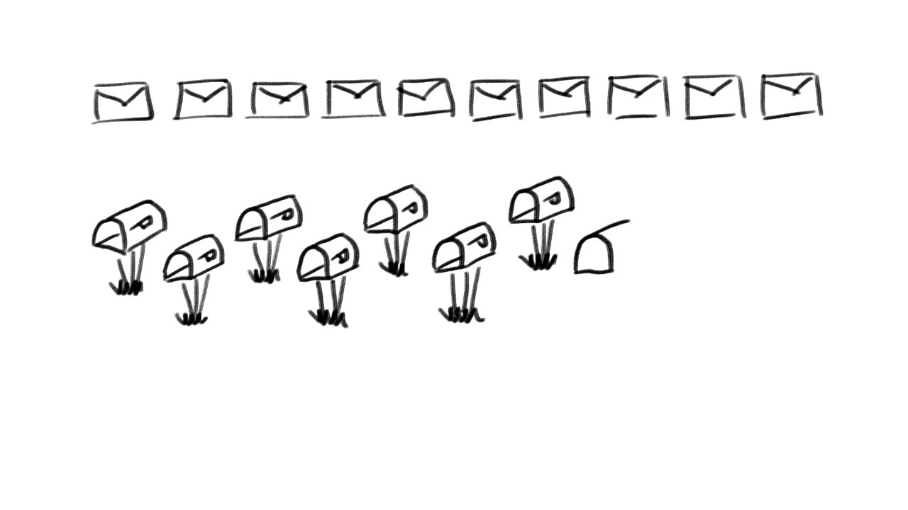
2:53 let's look at a mail carrier as an
2:55 example in a town with only one person
2:58 and one letter to deliver
2:59 the genie impurity would be equal to
3:01 zero since there's no chance of being
3:03 incorrect
3:04 however if there are 10 people in the
3:07 town with one letter for each
3:09 the impurity would be 0.9 because
3:12 now there's a 1 in 10 chance of placing
3:15 the randomly selected mail into the
3:16 right mailbox
3:19 information gain helps us find the
3:20 question that reduces our uncertainty
3:22 the most
3:24 it's just a number that tells us how
3:25 much a question helps to unmix the
3:27 labels at a node
3:29 we begin by calculating the uncertainty
3:31 of our starting set
3:33 impurity equals 0.48 then for each
3:37 question we segment the data
3:38 and calculate the uncertainty of the
3:40 child nodes
3:41 we take a weighted average of their
3:43 uncertainty because we care more about a
3:45 large set
3:46 with low uncertainty than a small set
3:48 with high uncertainty
3:49 then we subtract that from our starting
3:51 uncertainty and that's our information
3:53 gain
3:54 as we continue we'll keep track of the
3:56 question with the most gain
3:57 and that will be the best one to ask at
3:59 this node
4:01 now we're ready to build the tree we
4:03 start at the root node of the tree which
4:05 is given the entire data set
4:07 then we need the best question to ask at
4:09 this node
4:10 we find this by iterating over each of
4:13 these values
4:14 we split the data and calculate the
4:16 information gain for each one
4:18 as we go we keep track of the question
4:20 that produces the most gain
4:22 found it once we find the most useful
4:24 question to ask we split the data using
4:27 this question
4:28 we then add a child node to this branch
4:30 and it uses the subset of data after the
4:32 split
4:33 again we calculate the information gain
4:36 to discover the best question for this
4:37 data
4:39 rinse and repeat until there are no
4:40 further questions to ask
4:42 and this node becomes a leaf which
4:44 provides the final prediction
4:47 we hope this gives you insight into the
4:48 ai we've created
4:50 if you'd like to see more from a
4:51 practical perspective visit our
4:53 solutions page on juniper.net

